One of the jobs that all teachers have in common is evaluating students. Whether you use exams, homework assignments, quizzes, or projects, you usually have to turn students’ scores into a letter grade at the end of the term. This often involves a bunch of calculations that you might do in a spreadsheet. Instead, you can consider using Python and pandas.
One problem with using a spreadsheet is that it can be hard to see when you make a mistake in a formula. Maybe you selected the wrong column and put quizzes where exams should go. Maybe you found the maximum of two incorrect values. To solve this problem, you can use Python and pandas to do all your calculations and find and fix those mistakes much faster.
In this tutorial, you’ll learn how to:
- Load and merge data from multiple sources with pandas
- Filter and group data in a pandas DataFrame
- Calculate and plot grades in a pandas DataFrame
Click the link below to download the code for this pandas project and follow along as you build your gradebook script:
Get the Source Code: Click here to get the source code you’ll use to build a gradebook with pandas in this tutorial.
Build It: In this tutorial, you’ll build a full project from start to finish. If you’d like to learn more about pandas, then check out the pandas learning path.
Demo: What You’ll Build
In this pandas project, you’re going to create a Python script that loads your grade data and calculates letter grades for your students. Check out this video for a demonstration of the script in action:

Your script will run from the command line or your IDE and will produce CSV output files so you can paste the grades into your school’s grading system. You’ll also produce a few plots to take a look at how your grades are distributed.
Project Overview
This pandas project involves four main steps:
- Explore the data you’ll use in the project to determine which format and data you’ll need to calculate your final grades.
- Load the data into pandas DataFrames, making sure to connect the grades for the same student across all your data sources.
- Calculate the final grades and save them as CSV files.
- Plot the grade distribution and explore how the grades vary among your students.
Once you complete these steps, you’ll have a working Python script that can calculate your grades. Your grades will be in a format that you should be able to upload to your school’s student administration system.
Background Reading
You’ll get the most out of this pandas project if you have a little bit of experience working with pandas. If you need a refresher, then these tutorials and courses will get you up to speed for this project:
- The Pandas DataFrame: Make Working With Data Delightful
- Basic Pandas Data Structures
- Pandas: How to Read and Write Files
- Reading CSVs With Pandas
- Combining Data in Pandas With
merge(),.join(), andconcat()
Don’t worry too much about memorizing all the details in those tutorials. You’ll see a practical application of the topics in this pandas project. Now let’s take a look at the data you’ll be using in this project!
Exploring the Data for This Pandas Project
Like most teachers, you probably used a variety of services to manage your class this term, including:
- The school’s student administration system
- A service to manage assigning and grading homework and exams
- A service to manage assigning and grading quizzes
For the purposes of this project, you’ll use sample data that represents what you might get out of these systems. The data is in comma-separated values (CSV) files. Some samples of the data are shown here. First, there’s a file that contains the roster information for the class. This would come from your student administration system:
| ID | Name | NetID | Email Address | Section |
|---|---|---|---|---|
| 1234567 | “Barrera Jr., Woody” | WXB12345 | WOODY.BARRERA_JR@UNIV.EDU | 1 |
| 2345678 | “Lambert, Malaika” | MXL12345 | MALAIKA.LAMBERT@UNIV.EDU | 2 |
| 3456789 | “Joyce, Traci” | TXJ12345 | TRACI.JOYCE@UNIV.EDU | 1 |
| 4567890 | “Flower, John Gregg” | JGF12345 | JOHN.G.2.FLOWER@UNIV.EDU | 3 |
This table indicates each student’s ID number, name, NetID, and email address as well as the section of the class that they belong to. In this term, you taught one class that met at different times, and each class time has a different section number.
Next, you have a file that contains homework and exam scores. This one is from the homework and exam grading service and has a slightly different arrangement of columns than the roster:
| SID | First Name | Last Name | Homework 1 | Homework 1 - Max Points | Homework 1 - Submission Time | … |
|---|---|---|---|---|---|---|
| jgf12345 | Gregg | Flower | 69 | 80 | 2019-08-29 08:56:02-07:00 | … |
| mxl12345 | Malaika | Lambert | 63 | 80 | 2019-08-29 08:56:02-07:00 | … |
| txj12345 | Traci | Joyce | 80 | 2019-08-29 08:56:02-07:00 | … | |
| wxb12345 | Woody | Barrera | 55 | 80 | 2019-08-29 08:56:02-07:00 | … |
In this table, each student has an SID, first name, and last name. In addition, there are three values reported for each homework assignment and exam you gave:
- The score the student received
- The maximum score for that assignment
- The time the student submitted the assignment
Last, you have files that contain information for quiz grades. These files are separated so that one quiz is stored in each data file, and the information in these files is different from the roster and the homework files:
| Last Name | First Name | Grade | |
|---|---|---|---|
| Barrera | Woody | woody.barrera_jr@univ.edu | 4 |
| Flower | John | john.g.2.flower@univ.edu | 8 |
| Joyce | Traci | traci.joyce@univ.edu | 8 |
| Lambert | Malaika | malaika.lambert@univ.edu | 8 |
In the quiz table, each student has a last name, first name, email, and quiz grade. Notice that the maximum possible quiz score isn’t stored in this table. You’ll see how to supply that information later on.
Inspecting this data, you might notice several features:
-
Each table has different representations of the students’ names. For instance, in the roster table the names are in the form
"Last Name, First Name"with quotes so that a CSV parser doesn’t interpret the comma as a new column. However, in the homework table, first names and last names each get their own column. -
Each student might use a different name in different data sources. For instance, the quiz tables don’t include the suffix
Jr.in Woody Barrera’s name. Another example is that John Flower prefers to be called by his middle name, Gregg, so he adjusted the display in the homework table. -
Each student’s email address doesn’t have the same elements. The basic email address for a student is
first.last@univ.edu. However, if an email of that form is already owned by another student, then the email address is modified to be unique. This means you can’t predict a student’s email address just from their name. -
Each column may use a unique name even if it has the same data. For instance, all the students have an identifier of the form
abc12345. The roster table calls this their NetID, while the homework table calls this their SID. The quiz tables don’t have this information at all. Similarly, some tables use the column headerEmail address, while others just useEmail. -
Each table sorts the data differently. In the roster table, the data are sorted by the
IDcolumn. In the homework table, the data are sorted by the first letter of the first name. In the quiz tables, the data are sorted in a random order. -
Each of the rows or columns in the tables may have missing data. For instance, Traci Joyce didn’t submit her work for Homework 1, so her row is blank in the homework table.
All of these features and more are present in data that you’ll see in the real world. In the rest of this pandas project, you’ll see how you can address each of these features and make sure they don’t disrupt your analysis.
Deciding on the Final Format for the Data
Now that you’ve seen the raw data formats, you can think about the final format of the data. In the end, you’ll need to calculate a letter grade for each student from their raw scores. Each row in your final data table will contain all the data for a single student. The number of rows will then be equal to the number of students in your class.
The columns will represent each homework score, quiz score, and exam score. You’ll also store some information about each student, including their name and unique identifier. Finally, you’ll store each of your calculations and the final letter grade in separate columns.
Here’s a sample of your final table:
| Identifier | Name | Homework | Quizzes | Exams | Final Score | Final Grade |
|---|---|---|---|---|---|---|
| Student 1 | Last, First | # | # | # | # | A–F |
| Student 2 | Last, First | # | # | # | # | A–F |
| … | … | … | … | … | … | … |
Each row in the table stores all the data for a single student. The first column has the student’s unique identifier and the second column has the student’s name. Then a series of columns stores the homework, quiz, exam, and final scores. Last is a column for the final grade.
Now that you’ve seen what the final shape of the data will be, you can get started working with the data. The first step is to load the data!
Loading the Data With Pandas
One of the best packages for working with tabular data in Python is pandas! You’re going to take advantage of a lot of the functionality in pandas, especially for merging datasets and performing mathematical operations with the data.
The code samples shown in this section are collected in the 01-loading-the-data.py file. You can download the source code by clicking the link below:
Get the Source Code: Click here to get the source code you’ll use to build a gradebook with pandas in this tutorial.
Create a Python script called gradebook.py. You’ll also need to create a folder called data that will store the input data files for your gradebook script.
Then, in gradebook.py, start by adding a module-level docstring that explains the purpose of the file. You can also import a few libraries right now:
"""Calculate student grades by combining data from many sources.

Using pandas, this script combines data from the:

* Roster
* Homework & Exam grades
* Quiz grades

to calculate final grades for a class.
"""
from pathlib import Path
import pandas as pd
In this code, you include a docstring that describes the purpose of the script. Then you import pathlib.Path and pandas.
Loading the Roster File
Now you’re ready to load the data, beginning with the roster:
HERE = Path(__file__).parent
DATA_FOLDER = HERE / "data"

roster = pd.read_csv(
    DATA_FOLDER / "roster.csv",
    converters={"NetID": str.lower, "Email Address": str.lower},
    usecols=["Section", "Email Address", "NetID"],
    index_col="NetID",
)
In this code, you create two constants, HERE and DATA_FOLDER, to keep track of the location of the currently executing file as well as the folder where the data is stored. These constants use the pathlib module to make it easy to refer to different folders.
Then you read the roster file using pd.read_csv(). To help process the data later, you set an index using index_col and include only the useful columns with usecols.
To make sure you can compare strings later, you also pass the converters argument to convert columns to lowercase. This will simplify the string comparisons you’ll do later on.
You can see some of the data in the roster DataFrame below:
| NetID | Email Address | Section |
|---|---|---|
| wxb12345 | woody.barrera_jr@univ.edu | 1 |
| mxl12345 | malaika.lambert@univ.edu | 2 |
| txj12345 | traci.joyce@univ.edu | 1 |
| jgf12345 | john.g.2.flower@univ.edu | 3 |
These are the first four rows from roster, and they match the rows from the roster table you looked at in the previous section. However, the NetID and Email Address columns have both been converted to lowercase strings because you passed str.lower to converters for those two columns. You’ve also omitted the Name and ID columns.
Loading the Homework and Exam File
Next, you can load the homework and exam grades CSV file. Remember that this file includes first and last names and the SID column in addition to all the grades. You want to ignore the columns with the submission times:
hw_exam_grades = pd.read_csv(
    DATA_FOLDER / "hw_exam_grades.csv",
    converters={"SID": str.lower},
    usecols=lambda x: "Submission" not in x,
    index_col="SID",
)
In this code, you again use the converters argument to convert the data in the SID and Email Address columns to lowercase. Although the data in these columns appear to be lowercase on first inspection, the best practice is to make sure that everything is consistent. You also need to specify SID as the index column to match the roster DataFrame.
In this CSV file, there are a number of columns containing assignment submission times that you won’t use in any further analysis. However, there are so many other columns that you want to keep that it would be tedious to list all of them explicitly.
To get around this, usecols also accepts functions that are called with one argument, the column name. If the function returns True, then the column is included. Otherwise, the column is excluded. With the lambda function you pass here, if the string "Submission" appears in the column name, then the column will be excluded.
Here’s a sample of the hw_exam_grades DataFrame to give you a sense of what the data looks like after it’s been loaded:
| SID | … | Homework 1 | Homework 1 - Max Points | Homework 2 | … |
|---|---|---|---|---|---|
| jgf12345 | … | 69 | 80 | 52 | … |
| mxl12345 | … | 63 | 80 | 57 | … |
| txj12345 | … | nan | 80 | 77 | … |
| wxb12345 | … | 55 | 80 | 62 | … |
These are the rows for the example students in the homework and exam grades CSV file you saw in the previous section. Notice that the missing data for Traci Joyce (SID txj12345) in the Homework 1 column was read as a nan, or Not a Number, value. You’ll see how to handle this kind of data in a later section. The ellipses (...) indicate columns of data that aren’t shown in the sample here but are loaded from the real data.
Loading the Quiz Files
Last, you need to load the data from the quizzes. There are five quizzes that you need to read, and the most useful form of this data is a single DataFrame rather than five separate DataFrames. The final data format will look like this:
| Quiz 5 | Quiz 2 | Quiz 4 | Quiz 1 | Quiz 3 | |
|---|---|---|---|---|---|
| woody.barrera_jr@univ.edu | 10 | 10 | 7 | 4 | 11 |
| john.g.2.flower@univ.edu | 5 | 8 | 13 | 8 | 8 |
| traci.joyce@univ.edu | 4 | 6 | 9 | 8 | 14 |
| malaika.lambert@univ.edu | 6 | 10 | 13 | 8 | 10 |
This DataFrame has the Email column as the index, and each quiz is in a separate column. Notice that the quizzes are out of order, but you’ll see when you calculate the final grades that the order doesn’t matter. You can use this code to load the quiz files:
quiz_grades = pd.DataFrame()
for file_path in DATA_FOLDER.glob("quiz_*_grades.csv"):
    quiz_name = " ".join(file_path.stem.title().split("_")[:2])
    quiz = pd.read_csv(
        file_path,
        converters={"Email": str.lower},
        index_col=["Email"],
        usecols=["Email", "Grade"],
    ).rename(columns={"Grade": quiz_name})
    quiz_grades = pd.concat([quiz_grades, quiz], axis=1)
In this code, you create an empty DataFrame called quiz_grades. You need the empty DataFrame for the same reason that you need to create an empty list before using list.append().
You use Path.glob() to find all the quiz CSV files and load them with pandas, making sure to convert the email addresses to lowercase. You also set the index column for each quiz to the students’ email addresses, which pd.concat() uses to align data for each student.
Notice that you pass axis=1 to pd.concat(). This causes pandas to concatenate columns rather than rows, adding each new quiz into a new column in the combined DataFrame.
Finally, you use DataFrame.rename() to change the name of the grade column from Grade to something specific to each quiz.
Merging the Grade DataFrames
Now that you have all your data loaded, you can combine the data from your three DataFrames, roster, hw_exam_grades, and quiz_grades. This lets you use one DataFrame for all your calculations and save a complete grade book to another format at the end.
All the modifications to gradebook.py made in this section are collected in the 02-merging-dataframes.py file. You can download the source code by clicking the link below:
Get the Source Code: Click here to get the source code you’ll use to build a gradebook with pandas in this tutorial.
You’ll merge the data together in two steps:
- Merge
rosterandhw_exam_gradestogether into a new DataFrame calledfinal_data. - Merge
final_dataandquiz_gradestogether.
You’ll use different columns in each DataFrame as the merge key, which is how pandas determines which rows to keep together. This process is necessary because each data source uses a different unique identifier for each student.
Merging the Roster and Homework Grades
In roster and hw_exam_grades, you have the NetID or SID column as a unique identifier for a given student. When merging or joining DataFrames in pandas, it’s most useful to have an index. You already saw how useful this was when you were loading the quiz files.
Remember that you passed the index_col argument to pd.read_csv() when you loaded the roster and the homework grades. Now you can merge these two DataFrames together:
final_data = pd.merge(
    roster, hw_exam_grades, left_index=True, right_index=True,
)
In this code, you use pd.merge() to combine the roster and hw_exam_grades DataFrames.
Here’s a sample of the merged DataFrame for the four example students:
| NetID | Email Address | … | Homework 1 | … |
|---|---|---|---|---|
| wxb12345 | woody.barrera_jr@univ.edu | … | 55 | … |
| mxl12345 | malaika.lambert@univ.edu | … | 63 | … |
| txj12345 | traci.joyce@univ.edu | … | nan | … |
| jgf12345 | john.g.2.flower@univ.edu | … | 69 | … |
Like you saw before, the ellipses indicate columns that aren’t shown in the sample here but are present in the actual DataFrame. The sample table shows that students with the same NetID or SID have been merged together, so their email addresses and Homework 1 grades match the tables you saw previously.
Merging the Quiz Grades
When you loaded the data for the quiz_grades, you used the email address as a unique identifier for each student. This is different from hw_exam_grades and roster, which used the NetID and SID, respectively.
To merge quiz_grades into final_data, you can use the index from quiz_grades and the Email Address column from final_data:
final_data = pd.merge(
    final_data, quiz_grades, left_on="Email Address", right_index=True
)
In this code, you use the left_on argument to pd.merge() to tell pandas to use the Email Address column in final_data in the merge. You also use right_index to tell pandas to use the index from quiz_grades in the merge.
Here’s a sample of the merged DataFrame showing the four example students:
| NetID | Email Address | … | Homework 1 | … | Quiz 3 |
|---|---|---|---|---|---|
| wxb12345 | woody.barrera_jr@univ.edu | … | 55 | … | 11 |
| mxl12345 | malaika.lambert@univ.edu | … | 63 | … | 10 |
| txj12345 | traci.joyce@univ.edu | … | nan | … | 14 |
| jgf12345 | john.g.2.flower@univ.edu | … | 69 | … | 8 |
Remember that ellipses mean that columns are missing in the sample table here but will be present in the merged DataFrame. You can double-check the previous tables to verify that the numbers are aligned for the correct students.
Filling in nan Values
Now all your data is merged into one DataFrame. Before you can move on to calculating the grades, you need to do one more bit of data cleaning.
You can see in the table above that Traci Joyce still has a nan value for her Homework 1 assignment. You can’t use nan values in calculations because, well, they’re not a number! You can use DataFrame.fillna() to assign a number to all the nan values in final_data:
final_data = final_data.fillna(0)
In this code, you use DataFrame.fillna() to fill all nan values in final_data with the value 0. This is an appropriate resolution because the nan value in Traci Joyce’s Homework 1 column indicates that the score is missing, meaning she probably didn’t hand in the assignment.
Here’s a sample of the modified DataFrame showing the four example students:
| NetID | … | First Name | Last Name | Homework 1 | … |
|---|---|---|---|---|---|
| wxb12345 | … | Woody | Barrera | 55 | … |
| mxl12345 | … | Malaika | Lambert | 63 | … |
| txj12345 | … | Traci | Joyce | 0 | … |
| jgf12345 | … | John | Flower | 69 | … |
As you can see in this table, Traci Joyce’s Homework 1 score is now 0 instead of nan, but the grades for the other students haven’t changed.
Calculating Grades With Pandas DataFrames
There are three categories of assignments that you had in your class:
- Exams
- Homework
- Quizzes
Each of these categories is assigned a weight toward the students’ final score. For your class this term, you assigned the following weights:
| Category | Percent of Final Grade | Weight |
|---|---|---|
| Exam 1 Score | 5 | 0.05 |
| Exam 2 Score | 10 | 0.10 |
| Exam 3 Score | 15 | 0.15 |
| Quiz Score | 30 | 0.30 |
| Homework Score | 40 | 0.40 |
The final score can be calculated by multiplying the weight by the total score from each category and summing all these values. The final score will then be converted to a final letter grade.
All the modifications to gradebook.py made in this section are collected in the 03-calculating-grades.py file. You can download the source code by clicking the link below:
Get the Source Code: Click here to get the source code you’ll use to build a gradebook with pandas in this tutorial.
This means that you have to calculate the total from each category. The total from each category is a floating-point number from 0 to 1 that represents how many points a student earned relative to the maximum possible score. You’ll handle each assignment category in turn.
Calculating the Exam Total Score
You’ll calculate grades for the exams first. Since each exam has a unique weight, you can calculate the total score for each exam individually. It makes the most sense to use a for loop, which you can see in this code:
n_exams = 3
for n in range(1, n_exams + 1):
    final_data[f"Exam {n} Score"] = (
        final_data[f"Exam {n}"] / final_data[f"Exam {n} - Max Points"]
    )
In this code, you set n_exams equal to 3 because you had three exams during the term. Then you loop through each exam to calculate the score by dividing the raw score by the max points for that exam.
Here’s a sample of the exam data for the four example students:
| NetID | Exam 1 Score | Exam 2 Score | Exam 3 Score |
|---|---|---|---|
| wxb12345 | 0.86 | 0.62 | 0.90 |
| mxl12345 | 0.60 | 0.91 | 0.93 |
| txj12345 | 1.00 | 0.84 | 0.64 |
| jgf12345 | 0.72 | 0.83 | 0.77 |
In this table, each student scored between 0.0 and 1.0 on each of the exams. At the end of your script, you’ll multiply these scores by the weight to determine the proportion of the final grade.
Calculating the Homework Scores
Next, you need to calculate the homework scores. The max points for each homework assignment varies from 50 to 100. This means that there are two ways to calculate the homework score:
- By total score: Sum the raw scores and maximum points independently, then take the ratio.
- By average score: Divide each raw score by its respective maximum points, then take the sum of these ratios and divide the total by the number of assignments.
The first method gives a higher score to students who performed consistently, while the second method favors students who did well on assignments that were worth more points. To help students, you’ll give them the maximum of these two scores.
Computing these scores will take a few steps:
- Collect the columns with homework data.
- Compute the total score.
- Compute the average score.
- Determine which score is larger and will be used in the final score calculation.
First, you need to collect all the columns with homework data. You can use DataFrame.filter() to do this:
homework_scores = final_data.filter(regex=r"^Homework \d\d?$", axis=1)
homework_max_points = final_data.filter(regex=r"^Homework \d\d? -", axis=1)
In this code, you use a regular expression (regex) to filter final_data. If a column name doesn’t match the regex, then the column won’t be included in the resulting DataFrame.
The other argument you pass to DataFrame.filter() is axis. Many methods of a DataFrame can operate either row-wise or column-wise, and you can switch between the two approaches using the axis argument. With the default argument axis=0, pandas would look for rows in the index that match the regex you passed. Since you want to find all the columns that match the regex instead, you pass axis=1.
Now that you’ve collected the columns you need from the DataFrame, you can do the calculations with them. First, you sum the two values independently and then divide them to compute the total homework score:
sum_of_hw_scores = homework_scores.sum(axis=1)
sum_of_hw_max = homework_max_points.sum(axis=1)
final_data["Total Homework"] = sum_of_hw_scores / sum_of_hw_max
In this code, you use DataFrame.sum() and pass the axis argument. By default, .sum() will add up the values for all the rows in each column. However, you want the sum of all the columns for each row because each row represents one student. The axis=1 argument tells pandas to do just that.
Then you assign a new column in final_data called Total Homework to the ratio of the two sums.
Here’s a sample of the calculation results for the four example students:
| NetID | Sum of Homework Scores | Sum of Max Scores | Total Homework |
|---|---|---|---|
| wxb12345 | 598 | 740 | 0.808108 |
| mxl12345 | 612 | 740 | 0.827027 |
| txj12345 | 581 | 740 | 0.785135 |
| jgf12345 | 570 | 740 | 0.770270 |
In this table, you can see the sum of the homework scores, the sum of the max scores, and the total homework score for each student.
The other calculation method is to divide each homework score by its maximum score, add up these values, and divide the total by the number of assignments. To do this, you could use a for loop and go through each column. However, pandas allows you to be more efficient because it will match column and index labels and perform mathematical operations only on matching labels.
To make this work, you need to change the column names for homework_max_points to match the names in homework_scores. You can do this using DataFrame.set_axis():
hw_max_renamed = homework_max_points.set_axis(homework_scores.columns, axis=1)
In this code, you create a new DataFrame, hw_max_renamed, and you set the columns axis to have the same names as the columns in homework_scores. Now you can use this DataFrame for more calculations:
average_hw_scores = (homework_scores / hw_max_renamed).sum(axis=1)
In this code, you calculate the average_hw_scores by dividing each homework score by its respective maximum points. Then you add the ratios together for all the homework assignments in each row with DataFrame.sum() and the argument axis=1.
Since the maximum value on each individual assignment is 1.0, the maximum value that this sum could take would equal the total number of homework assignments. However, you need a number that’s scaled from 0 to 1 to factor into the final grade.
This means you need to divide average_hw_scores by the number of assignments, which you can do with this code:
final_data["Average Homework"] = average_hw_scores / homework_scores.shape[1]
In this code, you use DataFrame.shape to get the number of assignments from homework_scores. Like a NumPy array, DataFrame.shape returns a tuple of (n_rows, n_columns). Taking the second value from the tuple gives you the number of columns in homework_scores, which is equal to the number of assignments.
Then you assign the result of the division to a new column in final_data called Average Homework.
Here’s a sample calculation result for the four example students:
| NetID | Sum of Average Homework Scores | Average Homework |
|---|---|---|
| wxb12345 | 7.99405 | 0.799405 |
| mxl12345 | 8.18944 | 0.818944 |
| txj12345 | 7.85940 | 0.785940 |
| jgf12345 | 7.65710 | 0.765710 |
In this table, notice that the Sum of Average Homework Scores can vary from 0 to 10, but the Average Homework column varies from 0 to 1. The second column will be used to compare to Total Homework next.
Now that you have your two homework scores calculated, you can take the maximum value to be used in the final grade calculation:
final_data["Homework Score"] = final_data[
    ["Total Homework", "Average Homework"]
].max(axis=1)
In this code, you select the two columns you just created, Total Homework and Average Homework, and assign the maximum value to a new column called Homework Score. Notice that you take the maximum for each student with axis=1.
Here’s a sample of the calculated results for the four example students:
| NetID | Total Homework | Average Homework | Homework Score |
|---|---|---|---|
| wxb12345 | 0.808108 | 0.799405 | 0.808108 |
| mxl12345 | 0.827027 | 0.818944 | 0.827027 |
| txj12345 | 0.785135 | 0.785940 | 0.785940 |
| jgf12345 | 0.770270 | 0.765710 | 0.770270 |
In this table, you can compare the Total Homework, Average Homework, and final Homework Score columns. You can see that the Homework Score always reflects the larger of Total Homework or Average Homework.
Calculating the Quiz Score
Next, you need to calculate the quiz score. The quizzes also have different numbers of maximum points, so you need to do the same procedure you did for the homework. The only difference is that the maximum grade on each quiz isn’t specified in the quiz data tables, so you need to create a pandas Series to hold that information:
quiz_scores = final_data.filter(regex=r"^Quiz \d$", axis=1)
quiz_max_points = pd.Series(
    {"Quiz 1": 11, "Quiz 2": 15, "Quiz 3": 17, "Quiz 4": 14, "Quiz 5": 12}
)

sum_of_quiz_scores = quiz_scores.sum(axis=1)
sum_of_quiz_max = quiz_max_points.sum()
final_data["Total Quizzes"] = sum_of_quiz_scores / sum_of_quiz_max

average_quiz_scores = (quiz_scores / quiz_max_points).sum(axis=1)
final_data["Average Quizzes"] = average_quiz_scores / quiz_scores.shape[1]

final_data["Quiz Score"] = final_data[
    ["Total Quizzes", "Average Quizzes"]
].max(axis=1)
Most of this code is quite similar to the homework code from the last section. The main difference from the homework case is that you created a pandas Series for quiz_max_points using a dictionary as input. The keys of the dictionary become index labels and the dictionary values become the Series values.
Since the index labels in quiz_max_points have the same names as quiz_scores, you don’t need to use DataFrame.set_axis() for the quizzes. pandas also broadcasts the shape of a Series so that it matches the DataFrame.
Here’s a sample of the result of this calculation for the quizzes:
| NetID | Total Quizzes | Average Quizzes | Quiz Score |
|---|---|---|---|
| wxb12345 | 0.608696 | 0.602139 | 0.608696 |
| mxl12345 | 0.681159 | 0.682149 | 0.682149 |
| txj12345 | 0.594203 | 0.585399 | 0.594203 |
| jgf12345 | 0.608696 | 0.615286 | 0.615286 |
In this table, the Quiz Score is always the larger of Total Quizzes or Average Quizzes, as expected.
Calculating the Letter Grade
Now you’ve completed all the required calculations for the final grade. You have scores for the exams, homework, and quizzes that are all scaled between 0 and 1. Next, you need to multiply each score by its weighting to determine the final grade. Then you can map that value onto a scale for letter grades, A through F.
Similar to the maximum quiz scores, you’ll use a pandas Series to store the weightings. That way, you can multiply by the correct columns from final_data automatically. Create your weightings with this code:
weightings = pd.Series(
    {
        "Exam 1 Score": 0.05,
        "Exam 2 Score": 0.1,
        "Exam 3 Score": 0.15,
        "Quiz Score": 0.30,
        "Homework Score": 0.4,
    }
)
In this code, you give a weighting to each component of the class. As you saw earlier, Exam 1 is worth 5 percent, Exam 2 is worth 10 percent, Exam 3 is worth 15 percent, quizzes are worth 30 percent, and Homework is worth 40 percent of the overall grade.
Next, you can combine these percentages with the scores you calculated previously to determine the final score:
final_data["Final Score"] = (final_data[weightings.index] * weightings).sum(
    axis=1
)
final_data["Ceiling Score"] = np.ceil(final_data["Final Score"] * 100)
In this code, you select the columns of final_data that have the same names as the index in weightings. You need to do this because some of the other columns in final_data have type str, so pandas will raise a TypeError if you try to multiply weightings by all of final_data.
Next, you take the sum of these columns for each student with DataFrame.sum(axis=1) and you assign the result of this to a new column called Final Score. The value in this column for each student is a floating-point number between 0 and 1.
Finally, being the really nice teacher that you are, you’re going to round each student’s grade up. You multiply each student’s Final Score by 100 to put it on a scale from 0 to 100, then you use numpy.ceil() to round each score to the next highest integer. You assign this value to a new column called Ceiling Score.
Note: You’ll have to add import numpy as np to the top of your script to use np.ceil().
Here’s a sample calculation result for these columns for the four example students:
| NetID | Final Score | Ceiling Score |
|---|---|---|
| wxb12345 | 0.745852 | 75 |
| mxl12345 | 0.795956 | 80 |
| txj12345 | 0.722637 | 73 |
| jgf12345 | 0.727194 | 73 |
The last thing to do is to map each student’s ceiling score onto a letter grade. At your school, you might use these letter grades:
- A: Score of 90 or higher
- B: Score between 80 and 90
- C: Score between 70 and 80
- D: Score between 60 and 70
- F: Score below 60
Since each letter grade has to map to a range of scores, you can’t easily use just a dictionary for the mapping. Fortunately, pandas has Series.map(), which allows you to apply an arbitrary function to the values in a Series. You could do something similar if you used a different grading scale than letter grades.
You can write an appropriate function this way:
grades = {
    90: "A",
    80: "B",
    70: "C",
    60: "D",
    0: "F",
}

def grade_mapping(value):
    for key, letter in grades.items():
        if value >= key:
            return letter
In this code, you create a dictionary that stores the mapping between the lower limit of each letter grade and the letter. Then you define grade_mapping(), which takes as an argument the value of a row from the ceiling score Series. You loop over the items in grades, comparing value to the key from the dictionary. If value is greater than key, then the student falls in that bracket and you return the appropriate letter grade.
Note: This function works only when the grades are arranged in descending order, and that relies on the order of the dictionary being maintained. If you’re using a version of Python older than 3.6, then you’ll need to use an OrderedDict instead.
With grade_mapping() defined, you can use Series.map() to find the letter grades:
letter_grades = final_data["Ceiling Score"].map(grade_mapping)
final_data["Final Grade"] = pd.Categorical(
    letter_grades, categories=grades.values(), ordered=True
)
In this code, you create a new Series called letter_grades by mapping grade_mapping() onto the Ceiling Score column from final_data. Since there are five choices for a letter grade, it makes sense for this to be a categorical data type. Once you’ve mapped the scores to letters, you can create a categorical column with the pandas Categorical class.
To create the categorical column, you pass the letter grades as well as two keyword arguments:
categoriesis passed the values fromgrades. The values ingradesare the possible letter grades in the class.orderedis passedTrueto tell pandas that the categories are ordered. This will help later if you want to sort this column.
The categorical column that you create is assigned to a new column in final_data called Final Grade.
Here are the final grades for the four example students:
| NetID | Final Score | Ceiling Score | Final Grade |
|---|---|---|---|
| wxb12345 | 0.745852 | 75 | C |
| mxl12345 | 0.795956 | 80 | B |
| txj12345 | 0.722637 | 73 | C |
| jgf12345 | 0.727194 | 73 | C |
Among the four example students, one person got a B and three people got Cs, matching their ceiling scores and the letter grade mapping you created.
Grouping the Data
Now that you’ve calculated the grades for each student, you probably need to put them into the student administration system. This term, you’re teaching several sections of the same class, as indicated by the Section column in the roster table.
All of the modifications to gradebook.py made in this section are collected in the 04-grouping-the-data.py file. You can download the source code by clicking the link below:
Get the Source Code: Click here to get the source code you’ll use to build a gradebook with pandas in this tutorial.
To put the grades into your student administration system, you need to separate the students into each section and sort them by their last name. Fortunately, pandas has you covered here as well.
pandas has powerful abilities to group and sort data in DataFrames. You need to group your data by the students’ section number and sort the grouped result by their name. You can do that with this code:
for section, table in final_data.groupby("Section"):
    section_file = DATA_FOLDER / f"Section {section} Grades.csv"
    num_students = table.shape[0]
    print(
        f"In Section {section} there are {num_students} students saved to "
        f"file {section_file}."
    )
    table.sort_values(by=["Last Name", "First Name"]).to_csv(section_file)
In this code, you use DataFrame.groupby() on final_data to group by the Section column and DataFrame.sort_values() to sort the grouped results. Last, you save the sorted data to a CSV file for upload to the student administration system. With that, you’re done with your grades for the term and you can relax for the break!
Plotting Summary Statistics
Before you hang up the whiteboard marker for the summer, though, you might like to see a little bit more about how the class did overall. Using pandas and Matplotlib, you can plot some summary statistics for the class.
All of the modifications made to gradebook.py in this section are collected in the 05-plotting-summary-statistics.py file. You can download the source code by clicking the link below:
Get the Source Code: Click here to get the source code you’ll use to build a gradebook with pandas in this tutorial.
First, you might want to see a distribution of the letter grades in the class. You can do that with this code:
grade_counts = final_data["Final Grade"].value_counts().sort_index()
grade_counts.plot.bar()
plt.show()
In this code, you use Series.value_counts() on the Final Grade column in final_data to calculate how many of each of the letters appear. By default, the value counts are sorted from most to fewest, but it would be more useful to see them in letter-grade order. You use Series.sort_index() to sort the grades into the order that you specified when you defined the Categorical column.
You then leverage pandas’s ability to use Matplotlib and produce a bar plot of the grade counts with DataFrame.plot.bar(). Since this is a script, you need to tell Matplotlib to show you the plot with plt.show(), which opens an interactive figure window.
Note: You’ll need to add import matplotlib.pyplot as plt at the top of your script for this to work.
Your figure should look similar to the figure below:
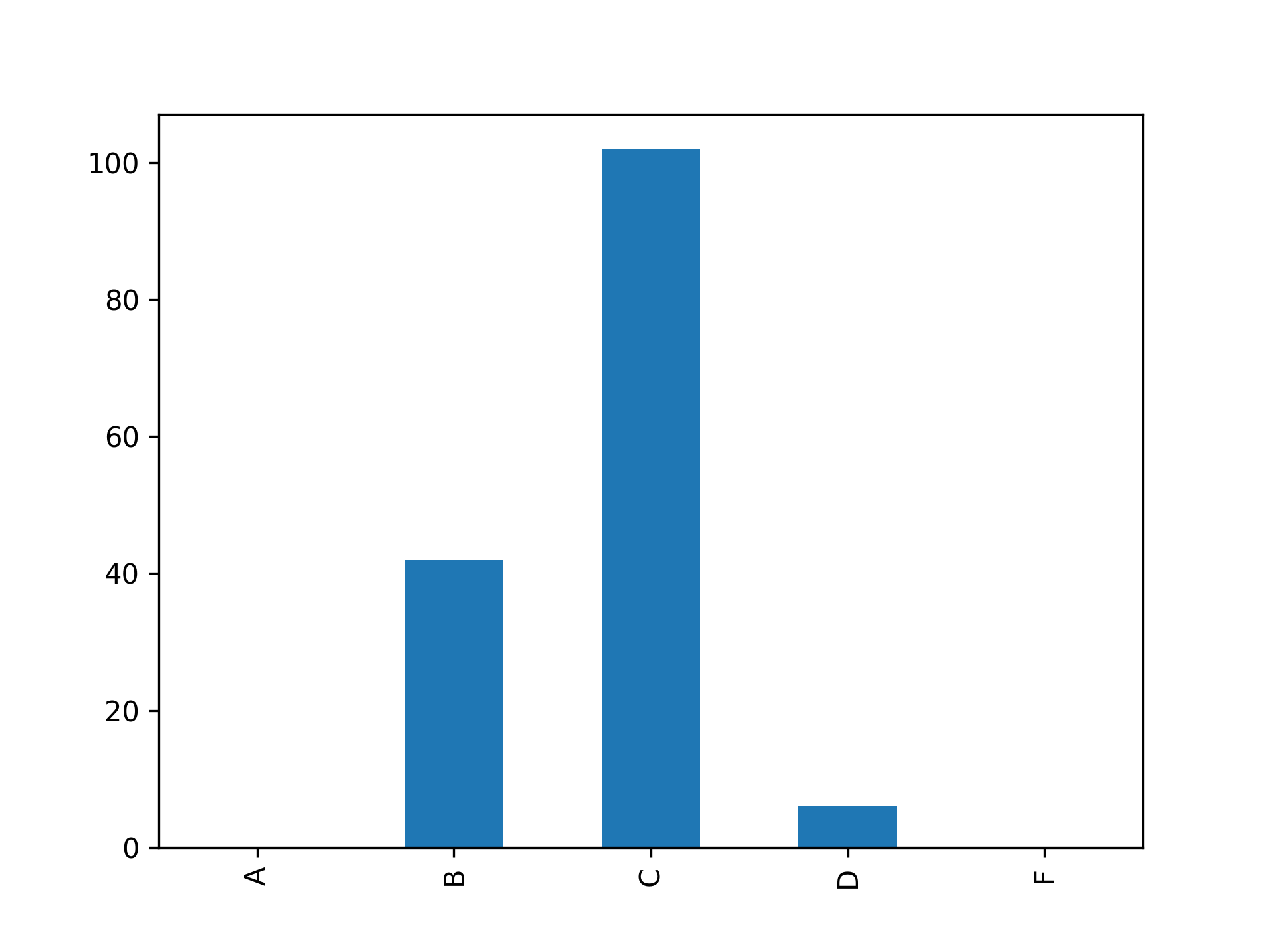
The height of the bars in this figure represents the number of students who received each letter grade shown on the horizontal axis. The majority of your students got a C letter grade.
Next, you might want to see a histogram of the numerical scores of the students. pandas can use Matplotlib with DataFrame.plot.hist() to do that automatically:
final_data["Final Score"].plot.hist(bins=20, label="Histogram")
In this code, you use DataFrame.plot.hist() to plot a histogram of the final scores. Any keyword arguments are passed through to Matplotlib when the plotting is done.
A histogram is one way to estimate the distribution of the data, but you might be interested in more sophisticated methods as well. pandas has the ability to use the SciPy library to calculate a kernel density estimate with DataFrame.plot.density(). You can also guess that the data will be normally distributed and manually calculate a normal distribution with the mean and standard deviation from your data. You can try this code to see how it works:
final_data["Final Score"].plot.density(
    linewidth=4, label="Kernel Density Estimate"
)

final_mean = final_data["Final Score"].mean()
final_std = final_data["Final Score"].std()
x = np.linspace(final_mean - 5 * final_std, final_mean + 5 * final_std, 200)
normal_dist = scipy.stats.norm.pdf(x, loc=final_mean, scale=final_std)
plt.plot(x, normal_dist, label="Normal Distribution", linewidth=4)
plt.legend()
plt.show()
In this code, you first use DataFrame.plot.density() to plot the kernel density estimate for your data. You adjust the line width and label for the plot to make it easier to see.
Next, you calculate the mean and standard deviation of your Final Score data using DataFrame.mean() and DataFrame.std(). You use np.linspace() to generate a set of x-values from -5 to +5 standard deviations away from the mean. Then you calculate the normal distribution in normal_dist by plugging into the formula for the standard normal distribution.
Note: You’ll need to add import scipy.stats at the top of your script for this to work.
Finally, you plot x vs normal_dist and adjust the line width and add a label. Once you show the plot, you should get a result that looks like this:
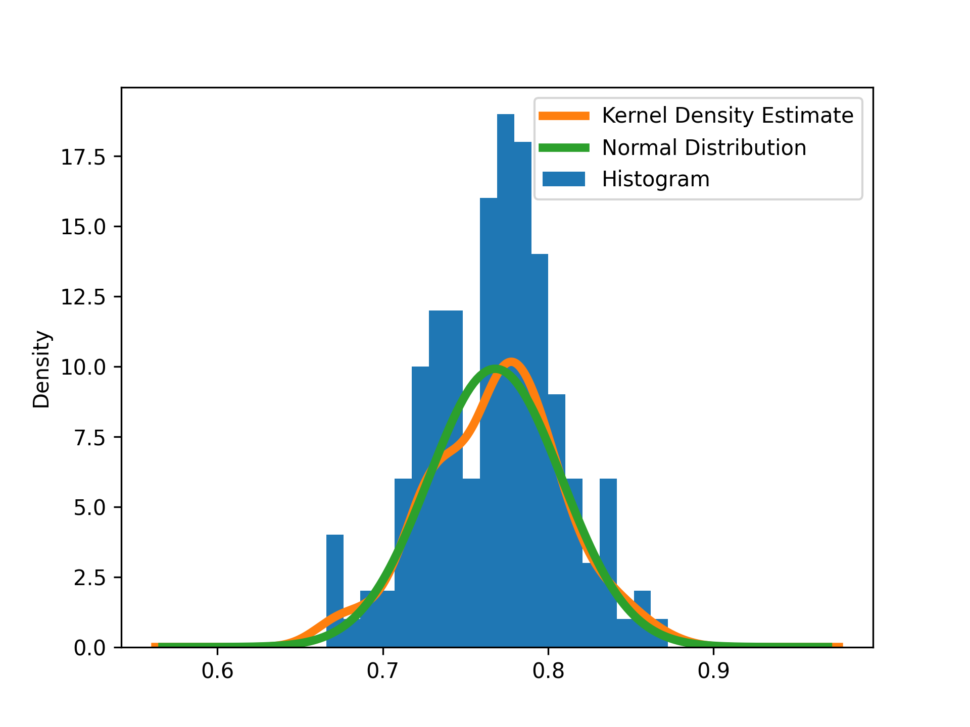
In this figure, the vertical axis shows the density of the grades in a particular bin. The peak occurs near a grade of 0.78. Both the kernel density estimate and the normal distribution do a pretty good job of matching the data.
Conclusion
You now know how to build a gradebook script with pandas so you can stop using spreadsheet software. This will help you avoid errors and calculate your final grades more quickly in the future.
In this tutorial, you learned:
- How to load, clean, and merge data into pandas DataFrames
- How to calculate with DataFrames and Series
- How to map values from one set to another
- How to plot summary statistics using pandas and Matplotlib
In addition, you saw how to group data and save files to upload to your student administration system. Now you’re ready to create your pandas gradebook for next term!
Click the link below to download the code for this pandas project and learn how to build a gradebook without spreadsheets:
Get the Source Code: Click here to get the source code you’ll use to build a gradebook with pandas in this tutorial.